Grid
This class generates a set of grid points. In a first step, the grid is always generated globally, with border a regional subset of points can be extracted from the global grid. The parameters R and inverseFlattening define the shape of the ellipsoid on which the grid is generated. In case inverseFlattening is chosen as zero, a sphere is used. With height the distance of the points above the ellipsoid can be defined. In addition to the location of the points, weights are assigned to each of the points. These weights can be regarded as the surface element associated with each grid point.
Geograph
The geographical grid is an equal-angular point distribution with points located along meridians and along circles of latitude. deltaLambda denotes the angular difference between adjacent points along meridians and deltaPhi describes the angular difference between adjacent points along circles of latitude. The point setting results as follows: \begin{equation} \lambda_i=\frac{\Delta\lambda}{2}+i\cdot\Delta\lambda\qquad\mbox{with}\qquad 0\leq i< \frac{360^\circ}{\Delta\lambda}, \end{equation}\begin{equation} \varphi_j=-90^\circ+\frac{\Delta\varphi}{2}+j\cdot\Delta\varphi\qquad\mbox{with}\qquad 0\leq j<\frac{180^\circ}{\Delta\varphi}. \end{equation}The number of grid points can be determined by \begin{equation} I=\frac{360^\circ}{\Delta\lambda}\cdot\frac{180^\circ}{\Delta\varphi}. \end{equation}The weights are calculated according to \begin{equation} w_i=\int\limits_{\lambda_i-\frac{\Delta\lambda}{2}}^{\lambda_i+\frac{\Delta\lambda}{2}}\int\limits_{\vartheta_i-\frac{\Delta\vartheta}{2}}^{\vartheta_i+\frac{\Delta\vartheta}{2}}=2\cdot\Delta\lambda\sin(\Delta\vartheta)\sin(\vartheta_i). \end{equation}
| Name | Type | Annotation |
|---|---|---|
deltaLambda | angle | |
deltaPhi | angle | |
height | double | ellipsoidal height expression (variables 'height', 'L', 'B') |
R | double | major axsis of the ellipsoid/sphere |
inverseFlattening | double | flattening of the ellipsoid, 0: sphere |
border | border |
TriangleVertex
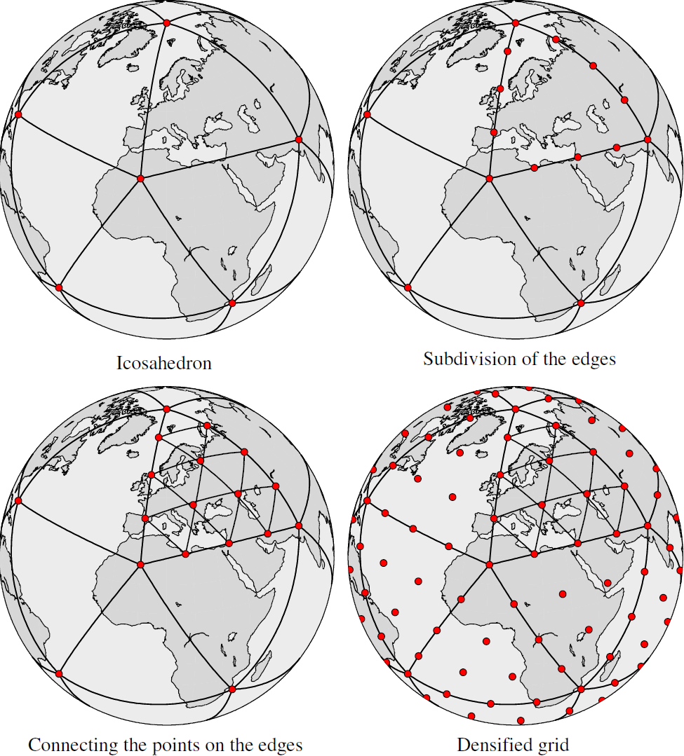
The zeroth level of densification
coincides with the 12 icosahedron vertices, as displayed in the upper left part
of Fig. fig:triangle_grid. Then, depending on the envisaged densification,
each triangle edge is divided into $n$ parts, illustrated in the upper right
part of Fig. fig:triangle_grid. The new nodes on the edges are then connected
by arcs of great circles parallel to the triangle edges. The intersections of
each three corresponding parallel lines become nodes of the densified grid as well.
As in case of a spherical triangle those three connecting lines do not exactly
intersect in one point, the center of the resulting triangle is used as location
for the new node (lower left part of Fig. fig:triangle_grid). The lower right
side of Fig. fig:triangle_grid finally shows the densified triangle vertex
grid for a level of $n=3$. The number of grid points in dependence of the chosen
level of densification can be calculated by
\begin{equation}\label{eq:numberVertex}
I=10\cdot(n+1)^2+2.
\end{equation}
| Name | Type | Annotation |
|---|---|---|
level | uint | division of icosahedron, point count = 10*(n+1)**2+2 |
R | double | major axsis of the ellipsoid/sphere |
inverseFlattening | double | flattening of the ellipsoid, 0: sphere |
border | border |
TriangleCenter
The points of the zeroth level are located at the centers of the icosahedron triangles. To achieve a finer grid, each of the triangles is divided into four smaller triangles by connecting the midpoints of the triangle edges. The refined grid points are again located at the center of the triangles. Subsequently, the triangles can be further densified up to the desired level of densification $n$, which is defined by level.
The number of global grid points for a certain level can be determined by \begin{equation}\label{eq:numberCenter} I=20\cdot 4^n. \end{equation}Thus the quantity of grid points depends exponentially on the level $n$, as with every additional level the number of grid points quadruplicates.
| Name | Type | Annotation |
|---|---|---|
level | uint | division of icosahedron, point count = 5*4**(n+1) |
R | double | major axsis of the ellipsoid/sphere |
inverseFlattening | double | flattening of the ellipsoid, 0: sphere |
border | border |
Gauss
The grid features equiangular spacing along circles of latitude with parallelsCount defining the number $L$ of the parallels. \begin{equation} \Delta\lambda=\frac{\pi}{L}\qquad\Rightarrow\qquad\lambda_i=\frac{\Delta\lambda}{2}+i\cdot\Delta\lambda\qquad\mbox{with}\qquad 0\leq i< 2L. \end{equation}Along the meridians the points are located at $L$ parallels at the $L$ zeros $\vartheta_j$ of the Legendre polynomial of degree $L$, \begin{equation} P_L(\cos\vartheta_j)=0. \end{equation}Consequently, the number of grid points sums up to \begin{equation} I=2\cdot L^2. \end{equation}The weights can be calculated according to \begin{equation} w_i(L)=\Delta\lambda\frac{2}{(1-t_i^2)(P'_{L}(\cos(\vartheta _i)))^2},\label{weights} \end{equation}
| Name | Type | Annotation |
|---|---|---|
parallelsCount | uint | |
R | double | major axsis of the ellipsoid/sphere |
inverseFlattening | double | flattening of the ellipsoid, 0: sphere |
border | border |
Reuter
The Reuter grid features equi-distant spacing along the meridians determined by the control parameter $\gamma$ according to \begin{equation} \Delta\vartheta=\frac{\pi}{\gamma}\qquad\Rightarrow\vartheta_j=j\Delta\vartheta,\qquad\mbox{with}\qquad 1\leq j\leq \gamma-1. \end{equation}Thus $\gamma+1$ denotes the number of points per meridian, as the two poles are included in the point distribution as well. Along the circles of latitude, the number of grid points decreases with increasing latitude in order to achieve an evenly distributed point pattern. This number is chosen, so that the points along each circle of latitude have the same spherical distance as two adjacent latitudes. The resulting relationship is given by \begin{equation}\label{eq:sphericalDistance} \Delta\vartheta=\arccos\left( \cos^2\vartheta_j+\sin^2\vartheta_j\cos\Delta\lambda_j\right). \end{equation}The left hand side of this equation is the spherical distance between adjacent latitudes, the right hand side stands for the spherical distance between two points with the same polar distance $\vartheta_j$ and a longitudinal difference of $\Delta\lambda_i$. This longitudinal distance can be adjusted depending on $\vartheta_j$ to fulfill Eq. \eqref{eq:sphericalDistance}. The resulting formula for $\Delta\lambda_i$ is \begin{equation}\label{eq:deltaLambdai} \Delta\lambda_j=\arccos\left( \frac{\sin\Delta\vartheta -\cos^2\vartheta_j}{\sin^2\vartheta_j}\right). \end{equation}The number of points $\gamma_j$ for each circle of latitude can then be determined by \begin{equation}\label{eq:gammai} \gamma_j=\left[ \frac{2\pi}{\Delta\lambda_j}\right] . \end{equation}Here the Gauss bracket $[x]$ specifies the largest integer equal to or less than $x$. The longitudes are subsequently determined by \begin{equation} \lambda_{ij}=\frac{\Delta\lambda_j}{2}+i\cdot(2\pi/\gamma_j),\qquad\mbox{with}\qquad 0\leq i< \gamma_j. \end{equation}The number of grid points can be estimated by \begin{equation}\label{eq:numberReuter} I=\leq 2+\frac{4}{\pi}\gamma^2, \end{equation}The $\leq$ results from the fact that the $\gamma_j$ are restricted to integer values.
| Name | Type | Annotation |
|---|---|---|
gamma | uint | number of parallels |
height | double | ellipsoidal height |
R | double | major axsis of the ellipsoid/sphere |
inverseFlattening | double | flattening of the ellipsoid, 0: sphere |
border | border |
Corput
This kind of grid distributes an arbitrarily chosen number of $I$ points (defined by globalPointsCount) following a recursive, quasi random sequence. In longitudinal direction the pattern follows \begin{equation} \Delta\lambda=\frac{2\pi}{I}\qquad\Rightarrow\qquad\frac{\Delta\lambda}{2}+\lambda_i=i\cdot\Delta\lambda\qquad\mbox{with}\qquad 1\leq i\leq I. \end{equation}This implies that every grid point features a unique longitude, with equi-angular longitudinal differences.
The polar distance in the form $t_i=\cos\vartheta_i$ for each point is determined by the following recursive sequence:
- Starting from an interval $t\in[-1,1]$.
- If $I=1$, then the midpoint of the interval is returned as result of the sequence, and the sequence is terminated.
- If the number of points is uneven, the midpoint is included into the list of $t_i$.
- Subsequently, the interval is bisected into an upper and lower half, and the sequence is called for both halves.
- $t$ from upper and lower half are alternately sorted into the list of $t_i$.
- The polar distances are calculated by \begin{equation} \vartheta_i=\arccos\, t_i. \end{equation}
| Name | Type | Annotation |
|---|---|---|
globalPointsCount | uint | |
height | double | ellipsoidal height |
R | double | major axsis of the ellipsoid/sphere |
inverseFlattening | double | flattening of the ellipsoid, 0: sphere |
border | border |
Driscoll
The Driscoll-Healy grid, has equiangular spacing along the meridians as well as along the circles of latitude. In longitudinal direction (along the parallels), these angular differences for a given dimension $L$ coincide with those described for the corresponding geographical grid and Gauss grid. Along the meridians, the size of the latitudinal differences is half the size compared to the geographical grid. This results in the following point pattern, \begin{equation} \begin{split} \Delta\lambda=\frac{\pi}{L}\qquad&\Rightarrow\qquad\lambda_i=\frac{\Delta\lambda}{2}+i\cdot\Delta\lambda\qquad&\mbox{with}\qquad 0\leq i< 2L, \\ \Delta\vartheta=\frac{\pi}{2L}\qquad&\Rightarrow\qquad\vartheta_j=j\cdot\Delta\vartheta\qquad&\mbox{with}\qquad 1\leq j\leq 2L. \end{split} \end{equation}Consequently, the number of grid points is \begin{equation} I=4\cdot L^2. \end{equation}The weights are given by \begin{equation} w_i=\Delta\lambda\frac{4}{2L}\sin(\vartheta_i)\sum_{l=0}^{L-1}\frac{\sin\left[ (2l+1)\;\vartheta_i\right] }{2l+1}. \end{equation}
| Name | Type | Annotation |
|---|---|---|
dimension | uint | number of parallels = 2*dimension |
height | double | ellipsoidal height |
R | double | major axsis of the ellipsoid/sphere |
inverseFlattening | double | flattening of the ellipsoid, 0: sphere |
border | border |
SinglePoint
Creates one single point.
| Name | Type | Annotation |
|---|---|---|
L | angle | longitude |
B | angle | latitude |
height | double | ellipsoidal height |
area | double | associated area element on unit sphere |
R | double | major axsis of the ellipsoid/sphere |
inverseFlattening | double | flattening of the ellipsoid, 0: sphere |
SinglePointCartesian
Creates one single point.
| Name | Type | Annotation |
|---|---|---|
x | double | [m] |
y | double | [m] |
z | double | [m] |
area | double | associated area element on unit sphere |
File
In this class grid is read from a file, which is given by inputfileGrid. A corresponding file can be generated with GriddedDataCreate or with Matrix2GriddedData.
| Name | Type | Annotation |
|---|---|---|
inputfileGrid | filename | |
border | border |